Display Settings for Elasticity Around the Hole View
The Display pane is accessed in the Elasticity Around the Hole view when you click on the Options ![]() button in the Elasticity View Toolbar. In the pane, you can modify the Visibility, Stereo plot options and the Failure zone options.
button in the Elasticity View Toolbar. In the pane, you can modify the Visibility, Stereo plot options and the Failure zone options.
 Visibility options
When you have selected multiple planes of weakness for the bedding planes, you can show or hide your families of fractures in the plot on the right side of the view using the check boxes under Bedding Planes.
You can show or hide the Stress Crosses on both the plots by checking the adjacent box. Stress crosses are the stress trajectories in a plane perpendicular to the borehole.
Show or hide the Breakout Position (from Caliper) on both the plots by checking the adjacent checkbox. By default, the breakout position from caliper log analysis are displayed in red. You can enter the deviation in depth (MD) of the breakout position from caliper data at the bottom of the form. For more information, see Integration of caliper analysis with borehole stress.
Stereo plot options
In this section, you control the Color scale and Contour settings of the stereo plot on the left side of the view. The Min and Max values of the color scale are shown in the entry boxes. For Log based calculation mode, these values are updated by default as you move the depth slider. You can also manually enter the values and, if needed, restore to default values using the  button.
- Color This is the default selection for the stereo plot on the left side of the view. For each Plot type, you can save a customized color scale range of Min and Max values. Use the 'Reverse color scale' checkbox on the plot to change the Min value to red and Max value to blue.
- Contour After selecting, the Options button underneath is activated. Click on the button to open the Contouring Options dialog. On the dialog, you have following options:
- Specify the contour Increments for the color scale range. Use the button to restore to default value.
- Select a Contour Type from the drop-down menu. There are three options: Contour, Overlay and Discrete Color. The Contour options show only the contours on the stereo plot without the continuous color scheme distribution on the borehole wall. Using Overlay displays the contours on top of the continuous color distribution on the plot. With the Discrete Color option, every increment in the range has a distinct color.
- Show labels Check the adjacent checkbox to show the contour labels on the plot. Click OK to save the settings on the dialog.
- Specify the contour Increments for the color scale range. Use the
Make sure you click the Refresh button to update the plot immediately each time you modify any settings in the Stereo plot options.
Display settings for the zone of failure
The four images below show the four different options for displaying the results when failure is defined in terms of the number of planes that would be predicted to slip, given the local stresses and pore pressure. The critical number of planes can be changed in the editable field so that you can see how the failure zone changes, as the number of slipping fracture sets changes. In general, the more sets slip, and the larger the area within which they slip, the more unstable the well is likely to be. For all examples, it is important to recognize that if no fracture plane actually penetrates a region within which it is predicted to slip, no failure will occur.
Image Example 1 shows that there is a fairly large zone within which any one of the fractures can slip. This can be thought of as the union of the regions within which each individual set can slip, so it could be quite large ( ). However, because only one of the fractures will slip, the rock within this zone is unlikely to wash out and fall into the hole.
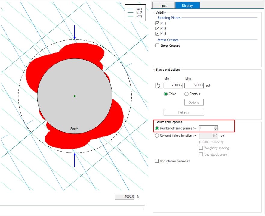
Example 1 of the Elasticity Around The Hole View, where any of the fractures can slip. click to enlarge
Image Example 2 shows the region within which at least two of the fractures could slip. This is a smaller region, as it is the union of the intersections of the regions within which pairs of fractures could slip ( ).
).
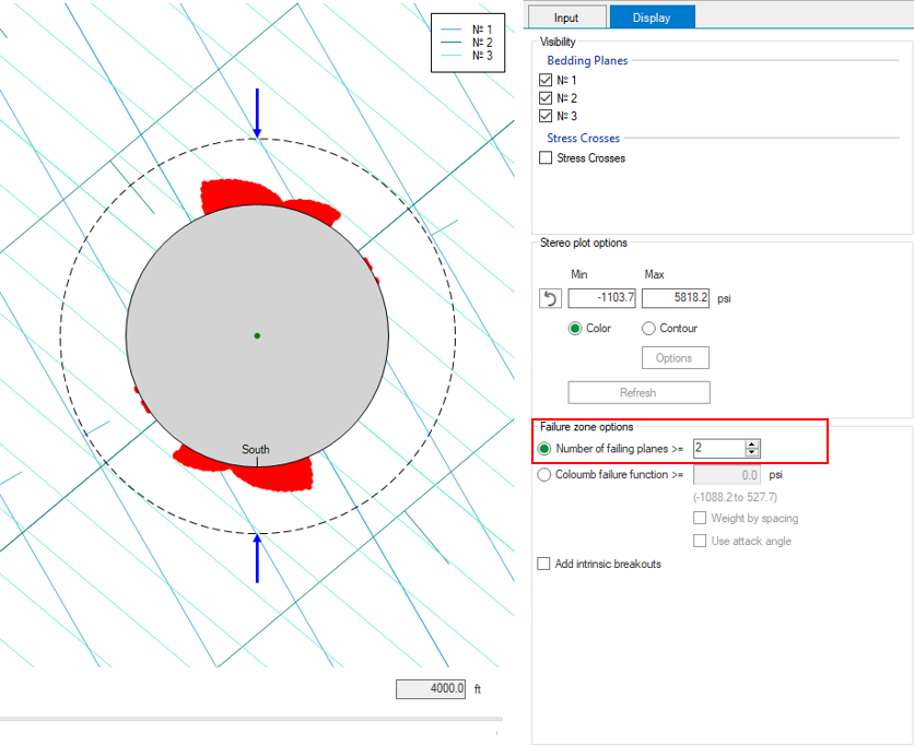
Example 2 of the Elasticity Around The Hole View, where at least two of the fractures can slip. click to enlarge
Image Example 3 shows the region within which all three of the fractures as defined would slip simultaneously. It is the smallest region, but it is also the region that it is most likely to create rubble that could fall into the well and cause drilling problems.
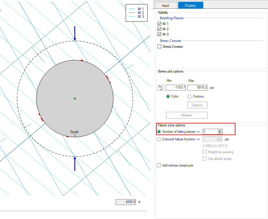
Example 3 of the Elasticity Around The Hole View, where all three fractures slip simultaneously. click to enlarge
Image Example 4 shows the combined zone within which all three fracture planes will slip and breakouts will occur because the intrinsic rock strength is exceeded by the stress concentration ( ).
).
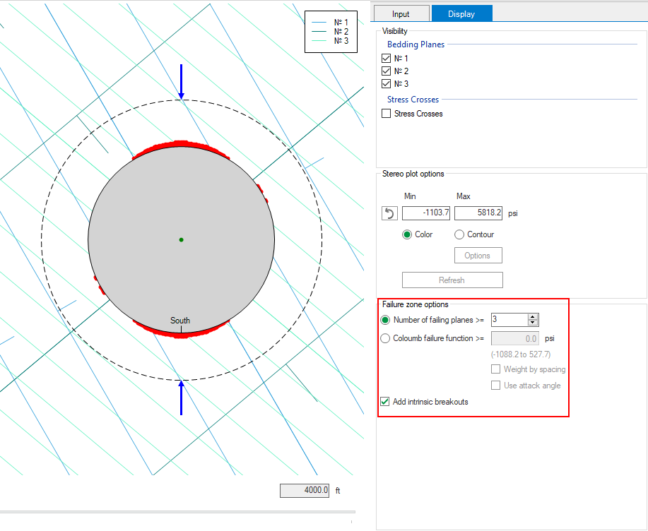
Example 4 of the Elasticity Around The Hole View, where all three fractures slip simultaneously and break out will occur. click to enlarge
Angle of attack
An alternative approach to evaluating the likelihood of failure is to compute, at each point around the well, the Coulomb Failure Function (CFF), which quantifies for a given stress state and fracture orientation how close that fracture is to slipping. CFF is explicitly defined for each fracture set as:

Here,
 is the resolved shear stress,
 is the sliding friction of the fracture,
 is the resolved effective normal stress, and
 is the cohesion of the fracture. The quantity
  is the shear stress for which the ith fracture would be in frictional equilibrium, so if
  is greater than zero the applied shear stress is larger than required for slip. In other words, for a given fracture, failure is defined as
  >0. The cumulative CFF is simply the sum of the CFF values for all of the fractures, or:

Fractures that are close together are more likely to be present in zones where they are predicted to fail, so it makes sense to weight the contributions of each fracture by their spacings. The weighted CFF is simply defined as

The spacing used to weight the individual CFFs is by default the number of fractures per unit length in space (the inverse of the perpendicular distance between adjacent fractures in the set). Different results are obtained if the weighting is based on the number of fractures that penetrate the well per unit well length. This number is the inverse of the fracture spacing times the square of the cosine of the angle (called the attack angle) between the fracture normal and the wellbore axis. Thus, planes parallel to the hole axis have zero weight regardless of their spacing, and planes perpendicular to the well have the maximum weight equal to their spacing.
To utilize CFF to define zones of failure around a well, select the Coulomb failure function in the Display tab from the setting options in the Around The Hole View. The result of selecting this display option is shown in the image below.
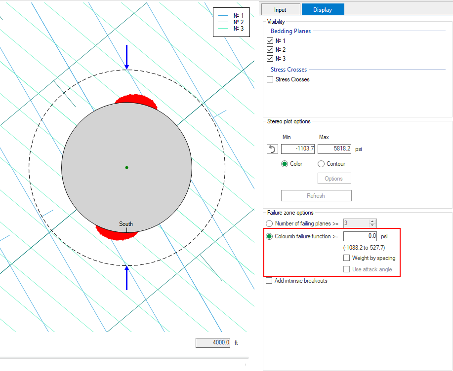
Example of the Elasticity Around The Hole View, CFF selected with default option: the criterion for failure is Cumulative CFF > 0. click to enlarge
You can change the default settings using the editable field under the Coulomb failure function radio button. The full range of CFF values is displayed below the editable field to guide you in choosing the appropriate limit.
To apply a weighting factor based on the fracture density, check the Weight by spacing check box. This creates an update of the output window, see image below.
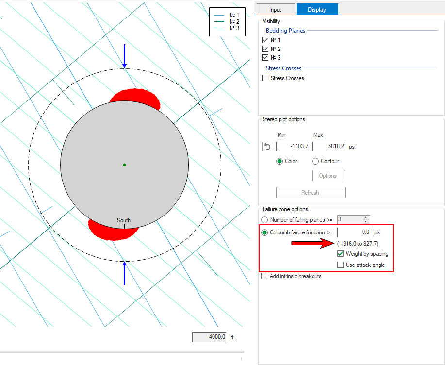
Example of the Elasticity Around The Hole View, CFF selected and weight by spacing. click to enlarge
The CFF is also updated with a different range of cumulative CFF and the Use attack angle checkbox is enabled.
Selecting the Use attack angle option results in the final output window, see image below. The range of CFF is again slightly different, as is the zone within which cumulative CFF exceeds the default value of zero selected using the editable field.
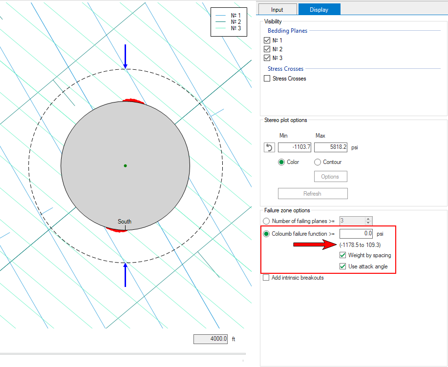
Example of the Elasticity Around The Hole View, CFF selected, weight by spacing and use attack angle. click to enlarge
If your solution has interpretation of breakout positions from the Caliper analysis, this option is activated. At the top of the form, you can select if you want to show or hide the breakout positions from caliper analysis. In this section, you enter the MD window (±) which indicates the deviation in the breakout position interpretation from caliper analysis.
Example showing the breakout position from caliper analysis with MD window of ±5 m along with the direction of maximum compression. click to enlarge